Apitrace maintenance

Lots of individuals and companies have made substantial contributions to Apitrace. But maintenance has always rested with me, the original author.

I would prefer have shared that responsibility with a wider team, but things haven't turned out that way. For several reasons I suppose:

• There are many people that care about one section of the functionality (one API, one OS), but few care about all of them.
• For all existing and potential contributors including me Apitrace is merely a means to an end (test/debug graphics drivers or applications), it's not an end on itself. The other stuff always gets the top priority.
• There are more polished tools for newer generation APIs like Vulkan, Metal, Direct3D 12. These newer APIs are much leaner than legacy APIs, which eliminates a lot of design constraints. And some of these tools have large teams behind them.
• Last but not least, I failed to nurture such a community. I always kept close control, partly to avoid things to become a hodgepodge, partly from fear of breakage, but can't shake the feeling that if I had been more relaxed things might of turned out differently.

Apitrace has always been something I worked on the spare time, or whenever I had an itch to scratch. That is still true, with the exception that after having a kid I have scarcely any free time left.

Furthermore the future is not bright: I believe Apitrace will have a long life in graphics driver test automation, and perhaps whenever somebody needs to debug an old OpenGL application, but I doubt it will flourish beyond that. And this facts weighs in whenever I need to decide whether to spend some time on Apitrace vs everything else.

The end result is that I haven't been a responsive maintainer for some time (long time merging patches, providing feedback, resolving issue, etc), and I'm afraid that will continue for the foreseeable future.

I don't feel any obligation to do more (after all, the license does say the software is provided as is), but I do want to set right expectations to avoid frustrating users/contributors who might otherwise timely feedback, hence this post.

Basic GLX_EXT_texture_from_pixmap support in ApiTrace

Apitrace now has basic support for the GLX_EXT_texture_from_pixmap extension, frequently used by Linux desktop compositors.

The difficulty with this extension was that it basically allows sharing textures between different processes, but when replaying those external processes and textures are not available. The solution was to emit fake glTexImage2D calls with the contents of the shared textures whenever they are used. (The same technique was already being for tracing OpenGL's GL_OES_EGL_image extension, and Direct3D's shared resources.)

This does yield large traces which are inadequate for profiling (something that can be eventually addressed with more effort.) But replays should be now visually faithful, therefore useful for debugging correctness/rendering issues.

Profiling OpenGL applications with ApiTrace

During the last 6 months I had the pleasure of supervising James Benton at VMware, for his industrial placement that is part of his course at Imperial College London.

Among other things, he added to support to ApiTrace for GPU profiling of OpenGL traces, and visualize both the captured GPU/CPU profiling results.

Visualization currently consists of a timeline showing calls start CPU/GPU time and durations, where GPU timings are grouped by the GLSL program bound:

And a histogram showing GPU/CPU durations for each call:

The interface was slightly retrouched since this screen-shots were taken.

Much more can be done (especially with cooperation from OpenGL driver developers to expose more GPU counters to OpenGL applications), but we are confident this new feature already can be quite handy for those looking for improving performance of their OpenGL applications.

James also designed a new homepage for ApiTrace on GitHub Pages. Please update your bookmarks!

ApiTrace 3.0

The Apitrace project came a long way since the first and last time I wrote about it here. One obvious reason is that I don't blog much (has it really been four years already!?). But the main reason is that this project received love from a lot of people since then, gaining features I could never dream of.

First, Zack Rusin implemented an awesome GUI and made writing/reading huge traces blazing fast.

Now, Carl Worth from Intel Linux Graphics Driver team implemented a top-level command, replacing the assortment of programs and scripts of with an unified command line interface, in the same spirit as git or Linux perf tool. He also added ability to trim traces, and is working on automatically trimming traces.

LunarG is developing several services based on Apitrace for GLES on Android and Chia-I Wu contributed back trace and retrace support for EGL, GLES1, and GLES2 APIs on Linux. Alexandros Frantzis from Linaro and Arnaud Vrac improved portability for embedded Linux platforms.

More goodies are bound to come soon, so stay tuned... to the github repository, not this blog! ;-)

Fast SSE2 pow: tables or polynomials?

We found that for many applications a substantial part of the time spent in software vertex processing was being spend in the powf function. So quite a few of us in Tungsten Graphics have been looking into a faster powf.

Introduction

The basic way to compute powf(x, y) efficiently is by computing the equivalent exp2(log2(x)*y)) expression, and then fiddle with IEEE 754 floating point exponent to quickly estimate the log2/exp2. This by itself only gives a very coarse approximation. To improve this approximation one has to also look into the mantissa, and then take one of two alternatives: use a lookup table or fit a function like a polynomial.

Lookup table

See also:

• Fast pow() With Adjustable Accuracy
• A fast logarithm implementation with adjustable accuracy

exp2

union f4 {
   int32_t i[4];
   uint32_t u[4];
   float f[4];
   __m128 m;
   __m128i mi;
};

#define EXP2_TABLE_SIZE_LOG2 9
#define EXP2_TABLE_SIZE (1 << EXP2_TABLE_SIZE_LOG2)
#define EXP2_TABLE_OFFSET (EXP2_TABLE_SIZE/2)
#define EXP2_TABLE_SCALE ((float) ((EXP2_TABLE_SIZE/2)-1))

/* 2 ^ x, for x in [-1.0, 1.0[ */
static float exp2_table[2*EXP2_TABLE_SIZE];

void exp2_init(void)
{
   int i;
   for (i = 0; i < EXP2_TABLE_SIZE; i++)
      exp2_table[i] = (float) pow(2.0, (i - EXP2_TABLE_OFFSET) / EXP2_TABLE_SCALE);
}

/**
 * Fast approximation to exp2(x).
 * Let ipart = int(x)
 * Let fpart = x - ipart;
 * So, exp2(x) = exp2(ipart) * exp2(fpart)
 * Compute exp2(ipart) with i << ipart
 * Compute exp2(fpart) with lookup table.
 */
__m128
exp2f4(__m128 x)
{
   __m128i ipart;
   __m128 fpart, expipart;
   union f4 index, expfpart;

   x = _mm_min_ps(x, _mm_set1_ps( 129.00000f));
   x = _mm_max_ps(x, _mm_set1_ps(-126.99999f));

   /* ipart = int(x) */
   ipart = _mm_cvtps_epi32(x);

   /* fpart = x - ipart */
   fpart = _mm_sub_ps(x, _mm_cvtepi32_ps(ipart));

   /* expipart = (float) (1 << ipart) */
   expipart = _mm_castsi128_ps(_mm_slli_epi32(_mm_add_epi32(ipart, _mm_set1_epi32(127)), 23));

   /* index = EXP2_TABLE_OFFSET + (int)(fpart * EXP2_TABLE_SCALE) */
   index.mi = _mm_add_epi32(_mm_cvtps_epi32(_mm_mul_ps(fpart, _mm_set1_ps(EXP2_TABLE_SCALE))), _mm_set1_epi32(EXP2_TABLE_OFFSET));

   expfpart.f[0] = exp2_table[index.u[0]];
   expfpart.f[1] = exp2_table[index.u[1]];
   expfpart.f[2] = exp2_table[index.u[2]];
   expfpart.f[3] = exp2_table[index.u[3]];

   return _mm_mul_ps(expipart, expfpart.m);
}

log2

#define LOG2_TABLE_SIZE_LOG2 8
#define LOG2_TABLE_SIZE (1 << LOG2_TABLE_SIZE_LOG2)
#define LOG2_TABLE_SCALE ((float) ((LOG2_TABLE_SIZE)-1))

/* log2(x), for x in [1.0, 2.0[ */
static float log2_table[2*LOG2_TABLE_SIZE];

void log2_init(void)
{
   unsigned i;
   for (i = 0; i < LOG2_TABLE_SIZE; i++)
      log2_table[i] = (float) log2(1.0 + i * (1.0 / (LOG2_TABLE_SIZE-1)));
}

__m128
log2f4(__m128 x)
{
   union f4 index, p;

   __m128i exp = _mm_set1_epi32(0x7F800000);
   __m128i mant = _mm_set1_epi32(0x007FFFFF);

   __m128i i = _mm_castps_si128(x);

   __m128 e = _mm_cvtepi32_ps(_mm_sub_epi32(_mm_srli_epi32(_mm_and_si128(i, exp), 23), _mm_set1_epi32(127)));

   index.mi = _mm_srli_epi32(_mm_and_si128(i, mant), 23 - LOG2_TABLE_SIZE_LOG2);

   p.f[0] = log2_table[index.u[0]];
   p.f[1] = log2_table[index.u[1]];
   p.f[2] = log2_table[index.u[2]];
   p.f[3] = log2_table[index.u[3]];

   return _mm_add_ps(p.m, e);
}

pow

static inline __m128
powf4(__m128 x, __m128 y)
{
   return exp2f4(_mm_mul_ps(log2f4(x), y));
}

Polynomial

For more details see:

• Posts from Nick from Ghent, Belgium in Approximate Math Library thread.
• Minimax Approximations and the Remez Algorithm

exp2

#define EXP_POLY_DEGREE 3

#define POLY0(x, c0) _mm_set1_ps(c0)
#define POLY1(x, c0, c1) _mm_add_ps(_mm_mul_ps(POLY0(x, c1), x), _mm_set1_ps(c0))
#define POLY2(x, c0, c1, c2) _mm_add_ps(_mm_mul_ps(POLY1(x, c1, c2), x), _mm_set1_ps(c0))
#define POLY3(x, c0, c1, c2, c3) _mm_add_ps(_mm_mul_ps(POLY2(x, c1, c2, c3), x), _mm_set1_ps(c0))
#define POLY4(x, c0, c1, c2, c3, c4) _mm_add_ps(_mm_mul_ps(POLY3(x, c1, c2, c3, c4), x), _mm_set1_ps(c0))
#define POLY5(x, c0, c1, c2, c3, c4, c5) _mm_add_ps(_mm_mul_ps(POLY4(x, c1, c2, c3, c4, c5), x), _mm_set1_ps(c0))

__m128 exp2f4(__m128 x)
{
   __m128i ipart;
   __m128 fpart, expipart, expfpart;

   x = _mm_min_ps(x, _mm_set1_ps( 129.00000f));
   x = _mm_max_ps(x, _mm_set1_ps(-126.99999f));

   /* ipart = int(x - 0.5) */
   ipart = _mm_cvtps_epi32(_mm_sub_ps(x, _mm_set1_ps(0.5f)));

   /* fpart = x - ipart */
   fpart = _mm_sub_ps(x, _mm_cvtepi32_ps(ipart));

   /* expipart = (float) (1 << ipart) */
   expipart = _mm_castsi128_ps(_mm_slli_epi32(_mm_add_epi32(ipart, _mm_set1_epi32(127)), 23));

   /* minimax polynomial fit of 2**x, in range [-0.5, 0.5[ */
#if EXP_POLY_DEGREE == 5
   expfpart = POLY5(fpart, 9.9999994e-1f, 6.9315308e-1f, 2.4015361e-1f, 5.5826318e-2f, 8.9893397e-3f, 1.8775767e-3f);
#elif EXP_POLY_DEGREE == 4
   expfpart = POLY4(fpart, 1.0000026f, 6.9300383e-1f, 2.4144275e-1f, 5.2011464e-2f, 1.3534167e-2f);
#elif EXP_POLY_DEGREE == 3
   expfpart = POLY3(fpart, 9.9992520e-1f, 6.9583356e-1f, 2.2606716e-1f, 7.8024521e-2f);
#elif EXP_POLY_DEGREE == 2
   expfpart = POLY2(fpart, 1.0017247f, 6.5763628e-1f, 3.3718944e-1f);
#else
#error
#endif

   return _mm_mul_ps(expipart, expfpart);
}

log2

#define LOG_POLY_DEGREE 5

__m128 log2f4(__m128 x)
{
   __m128i exp = _mm_set1_epi32(0x7F800000);
   __m128i mant = _mm_set1_epi32(0x007FFFFF);

   __m128 one = _mm_set1_ps( 1.0f);

   __m128i i = _mm_castps_si128(x);

   __m128 e = _mm_cvtepi32_ps(_mm_sub_epi32(_mm_srli_epi32(_mm_and_si128(i, exp), 23), _mm_set1_epi32(127)));

   __m128 m = _mm_or_ps(_mm_castsi128_ps(_mm_and_si128(i, mant)), one);

   __m128 p;

   /* Minimax polynomial fit of log2(x)/(x - 1), for x in range [1, 2[ */
#if LOG_POLY_DEGREE == 6
   p = POLY5( m, 3.1157899f, -3.3241990f, 2.5988452f, -1.2315303f,  3.1821337e-1f, -3.4436006e-2f);
#elif LOG_POLY_DEGREE == 5
   p = POLY4(m, 2.8882704548164776201f, -2.52074962577807006663f, 1.48116647521213171641f, -0.465725644288844778798f, 0.0596515482674574969533f);
#elif LOG_POLY_DEGREE == 4
   p = POLY3(m, 2.61761038894603480148f, -1.75647175389045657003f, 0.688243882994381274313f, -0.107254423828329604454f);
#elif LOG_POLY_DEGREE == 3
   p = POLY2(m, 2.28330284476918490682f, -1.04913055217340124191f, 0.204446009836232697516f);
#else
#error
#endif

   /* This effectively increases the polynomial degree by one, but ensures that log2(1) == 0*/
   p = _mm_mul_ps(p, _mm_sub_ps(m, one));

   return _mm_add_ps(p, e);
}

Results

The accuracy vs speed for several table sizes and polynomial degrees can be seen in the chart below.

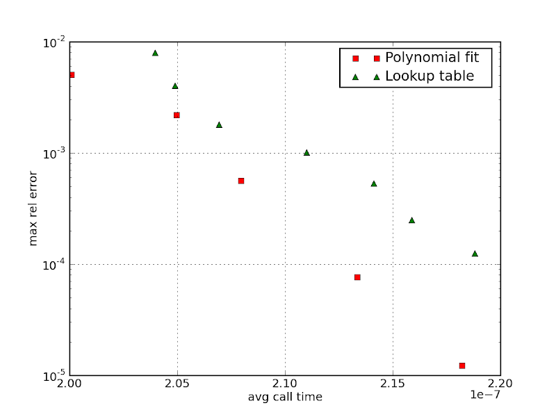
The difference is not much, but the polynomial approach outperforms the table approach for any desired precision. This was for 32bit generated code in a Core 2. If generating 64bit code, the difference between the two is bigger. The performance of the table approach will also tend to degrade when other computation is going on at the same time, as the likelihood the lookup tables get trashed out of the cache is higher. So by all accounts, the polynomial approach seems a safer bet.

Tracing Gallium3D

One nice thing about Gallium3D is that it provides a clean cut abstraction of (modern) 3D graphics hardware. The purpose of this abstraction is to allow a single hardware driver to target different graphic APIs (OpenGL, D3D, etc.). That is, one pipe driver for many state trackers.

But with this abstraction in place it opens the doors to other interesting things, unthinkable until now. Namely, by intercepting the calls between the state tracker and the pipe driver one could:

• in a debugging scenario, capture the calls of an application known to cause problems to a file and analyze it, replay it in order to isolate the bug;
• in a virtual machine scenario, capture all calls done inside a virtual machine and replay them in the host machine;
• in a performance analysis scenario, compute memory/performance statistics in a per-call/resource;
• etc.

Having an itch to scratch I started tackling the former, i.e., tracing Gallium3D for debugging purposes. Actually, an itch is an understatement, it is a rash named XP Direct3D. XP Direct3D driver model is in kernel space, and the build -> reboot -> upload driver -> test application cycle takes me between 5 and 10 min depending of the application. While in Linux building and testing from a NFS share takes me less than 1min. Recording a D3D application in XP and replay and debugging it on Linux would boost my productivity by 5 to 10 times. This assuming that the bug is on the pipe driver and not on the state tracker, which tends to be the case now that our state trackers are quite mature.

Using the learned lessons from my previous experiment of tracing D3D applications I wrote a pipe driver which traces all state tracker -> pipe driver interface calls to a XML file, and after an application written in Python to replay that file (using the Gallium3D Python bindings).

I chose a semantically rich XML as trace format so that the trace dumps are cross-platform and can at least survive minor interface changes such as addition/removal of state objects members, format renumbering, etc. This way traces can be also used for regression testing. Nevertheless the code is structured in such way that a space-efficient binary format is also possible in the future with minor changes.

Here is softpipe replaying a trace captured from trace of Mesa's gloss demo (also recorded on Linux).

Simple apps are capture/replayed (e.g., progs/trivial/*, progs/demos/gloss, and many D3D DirectX SDK examples), but big applications like 3DMark05 produce over 10GB of trace data before reaching the first frame, and I run out of disk space or patience before that. Also, some minor glitches in the interfaces prevent are causing some state to leak behind our back. So the next steps are to allow to capture a single arbitrary frame, improve trace format space efficiency, and trim the interface corners.

In case anybody gets interested, there are several README files in Mesa's git explaining how to use.

Learning and testing Gallium3D with Python

Gallium3D interfaces don't match any particular graphics API 1 to 1. Likewise, conformance tests end up not doing a good coverage of Gallium3D's interface either: sometimes a single Gallium3D feature is tested in many different tests; sometimes a feature ends up not being exercised by any test, so bugs are only detected in applications, where they are much harder to narrow down. And so appeared the need to write some tests at the Gallium3D interface level.

Since the ability to write tests quickly was important, and the running speed not so important, I've decided to write a Python bindings, so that tests could be scripted in Python. These bindings wrap around the pipe driver, so that they look like a pipe driver from the Python script point of view, and look like a state tracker from the pipe driver point of view.

About the tests there is not much to write about yet. I wrote tests for texture formats that allowed to squash the bugs I was searching for, and I imagine that more tests will be added as needs justify it.

However, having a Gallium3D bindings in Python opens several doors. One particularly is that it becomes a nice sandbox to learn Gallium3D. For example. here is the code to draw a single triangle:

def test(dev):
    ctx = dev.context_create()

    width = 255
    height = 255

    # disabled blending/masking
    blend = Blend()
    blend.rgb_src_factor = PIPE_BLENDFACTOR_ONE
    blend.alpha_src_factor = PIPE_BLENDFACTOR_ONE
    blend.rgb_dst_factor = PIPE_BLENDFACTOR_ZERO
    blend.alpha_dst_factor = PIPE_BLENDFACTOR_ZERO
    blend.colormask = PIPE_MASK_RGBA
    ctx.set_blend(blend)

    # no-op depth/stencil/alpha
    depth_stencil_alpha = DepthStencilAlpha()
    ctx.set_depth_stencil_alpha(depth_stencil_alpha)

    # rasterizer
    rasterizer = Rasterizer()
    rasterizer.front_winding = PIPE_WINDING_CW
    rasterizer.cull_mode = PIPE_WINDING_NONE
    rasterizer.bypass_clipping = 1
    rasterizer.scissor = 1
    #rasterizer.bypass_vs = 1
    ctx.set_rasterizer(rasterizer)

    # viewport (identity, we setup vertices in wincoords)
    viewport = Viewport()
    scale = FloatArray(4)
    scale[0] = 1.0
    scale[1] = 1.0
    scale[2] = 1.0
    scale[3] = 1.0
    viewport.scale = scale
    translate = FloatArray(4)
    translate[0] = 0.0
    translate[1] = 0.0
    translate[2] = 0.0
    translate[3] = 0.0
    viewport.translate = translate
    ctx.set_viewport(viewport)

    # samplers
    sampler = Sampler()
    sampler.wrap_s = PIPE_TEX_WRAP_CLAMP_TO_EDGE
    sampler.wrap_t = PIPE_TEX_WRAP_CLAMP_TO_EDGE
    sampler.wrap_r = PIPE_TEX_WRAP_CLAMP_TO_EDGE
    sampler.min_mip_filter = PIPE_TEX_MIPFILTER_NONE
    sampler.min_img_filter = PIPE_TEX_MIPFILTER_NEAREST
    sampler.mag_img_filter = PIPE_TEX_MIPFILTER_NEAREST
    sampler.normalized_coords = 1
    ctx.set_sampler(0, sampler)

    # scissor
    scissor = Scissor()
    scissor.minx = 0
    scissor.miny = 0
    scissor.maxx = width
    scissor.maxy = height
    ctx.set_scissor(scissor)

    clip = Clip()
    clip.nr = 0
    ctx.set_clip(clip)

    # framebuffer
    cbuf = dev.texture_create(
        PIPE_FORMAT_X8R8G8B8_UNORM, 
        width, height,
        tex_usage=PIPE_TEXTURE_USAGE_DISPLAY_TARGET,
    )
    _cbuf = cbuf.get_surface(usage = PIPE_BUFFER_USAGE_GPU_READ|PIPE_BUFFER_USAGE_GPU_WRITE)
    fb = Framebuffer()
    fb.width = width
    fb.height = height
    fb.num_cbufs = 1
    fb.set_cbuf(0, _cbuf)
    ctx.set_framebuffer(fb)
    _cbuf.clear_value = 0x00000000
    ctx.surface_clear(_cbuf, _cbuf.clear_value)
    del _cbuf
    
    # vertex shader
    vs = Shader('
        VERT1.1
        DCL IN[0], POSITION, CONSTANT
        DCL IN[1], COLOR, CONSTANT
        DCL OUT[0], POSITION, CONSTANT
        DCL OUT[1], COLOR, CONSTANT
        0:MOV OUT[0], IN[0]
        1:MOV OUT[1], IN[1]
        2:END
    ')
    ctx.set_vertex_shader(vs)

    # fragment shader
    fs = Shader('
        FRAG1.1
        DCL IN[0], COLOR, LINEAR
        DCL OUT[0], COLOR, CONSTANT
        0:MOV OUT[0], IN[0]
        1:END
    ')
    ctx.set_fragment_shader(fs)

    nverts = 3
    nattrs = 2
    verts = FloatArray(nverts * nattrs * 4)

    verts[ 0] = 128.0 # x1
    verts[ 1] =  32.0 # y1
    verts[ 2] =   0.0 # z1
    verts[ 3] =   1.0 # w1
    verts[ 4] =   1.0 # r1
    verts[ 5] =   0.0 # g1
    verts[ 6] =   0.0 # b1
    verts[ 7] =   1.0 # a1
    verts[ 8] =  32.0 # x2
    verts[ 9] = 224.0 # y2
    verts[10] =   0.0 # z2
    verts[11] =   1.0 # w2
    verts[12] =   0.0 # r2
    verts[13] =   1.0 # g2
    verts[14] =   0.0 # b2
    verts[15] =   1.0 # a2
    verts[16] = 224.0 # x3
    verts[17] = 224.0 # y3
    verts[18] =   0.0 # z3
    verts[19] =   1.0 # w3
    verts[20] =   0.0 # r3
    verts[21] =   0.0 # g3
    verts[22] =   1.0 # b3
    verts[23] =   1.0 # a3

    ctx.draw_vertices(PIPE_PRIM_TRIANGLES,
                      nverts, 
                      nattrs, 
                      verts)

    ctx.flush()

And this is the result:

In summary, you create several state atoms, bind them to the context, and then send the geometry through the pipe driver. Full source available in Mesa3D's git repository.

To use Gallium3D's Python bindings follow these instructions.

BTW, XDS 2008 is happening now. Too bad I couldn't go this year, as I would like to meet everybody. I hope you're having a great time!